Spice Model of a Mains Transformer

For my cistern wa­ter level meter, I al­so wanted to simulate the power supply unit, including the transformer.

It might seem unusual to simulate something so simp­le, but I recall early power supply designs from my days as a hobbyist where voltage regulators would shut down due to overheating, or ripple voltage from the filter capacitor would bleed through to the 5 V output because the voltage ahead of the regulator supplied by a 6 V transformer was simply too low.

Perhaps the situation could still be salvaged by increasing the size of the capacitor, or else the expensive transformer would have to be replaced with one having a higher secondary voltage...

Si­mu­la­tion doesn't cost much (just a little time), but it can save you a lot of trouble with the final circuit. You can see how the circuit behaves during a 15% undervoltage con­di­tion, measure power dissipation at 15% overvoltage as well as at no-load and maximum load, calculate the necessary heatsink, and so on.

The greatest source of uncertainty here is the mains transformer, since simulation data or parameters, let alone ready-made SPICE models, are typically unavailable for such components.

So we have to measure it ourselves. In my circuit, the component in question was a Gerth 387.15, a PCB-mount transformer rated for 15 V and 3.6 VA.

• The copper resistance of the windings
• The turns ratio
• The inductance of the windings

I have al­so included the resistance R_fe (representing hysteresis and eddy-current losses) and C_k (coupling capacitance), although these are negligible when using my stan­dard values. For reasons of symmetry, I split C_k into two capacitors. If you were able to measure these values, you can of course specify them as parameters.

The copper resistances can easily be determined using an ohmmeter.

The no-load turns ratio corresponds to the primary-to-secondary voltage ratio, which can be measured with any multimeter.

Determining the inductance, however, is somewhat problematic; because of saturation effects, it is not a constant value but depends on the voltage.

I am not aware of any truly accurate method for this that works with the power supply, multimeter, and oscilloscope typically found at hand.

I determined the inductance of the primary winding by connecting a 1 µF capacitor in pa­r­al­lel, exciting the resulting resonant circuit with 12 V and measuring the resonant frequency using an oscilloscope.

Since the inductances are pro­por­tio­nal to the square of the turns ratio, it follows that L_Sec=182 mH (not measured).

Here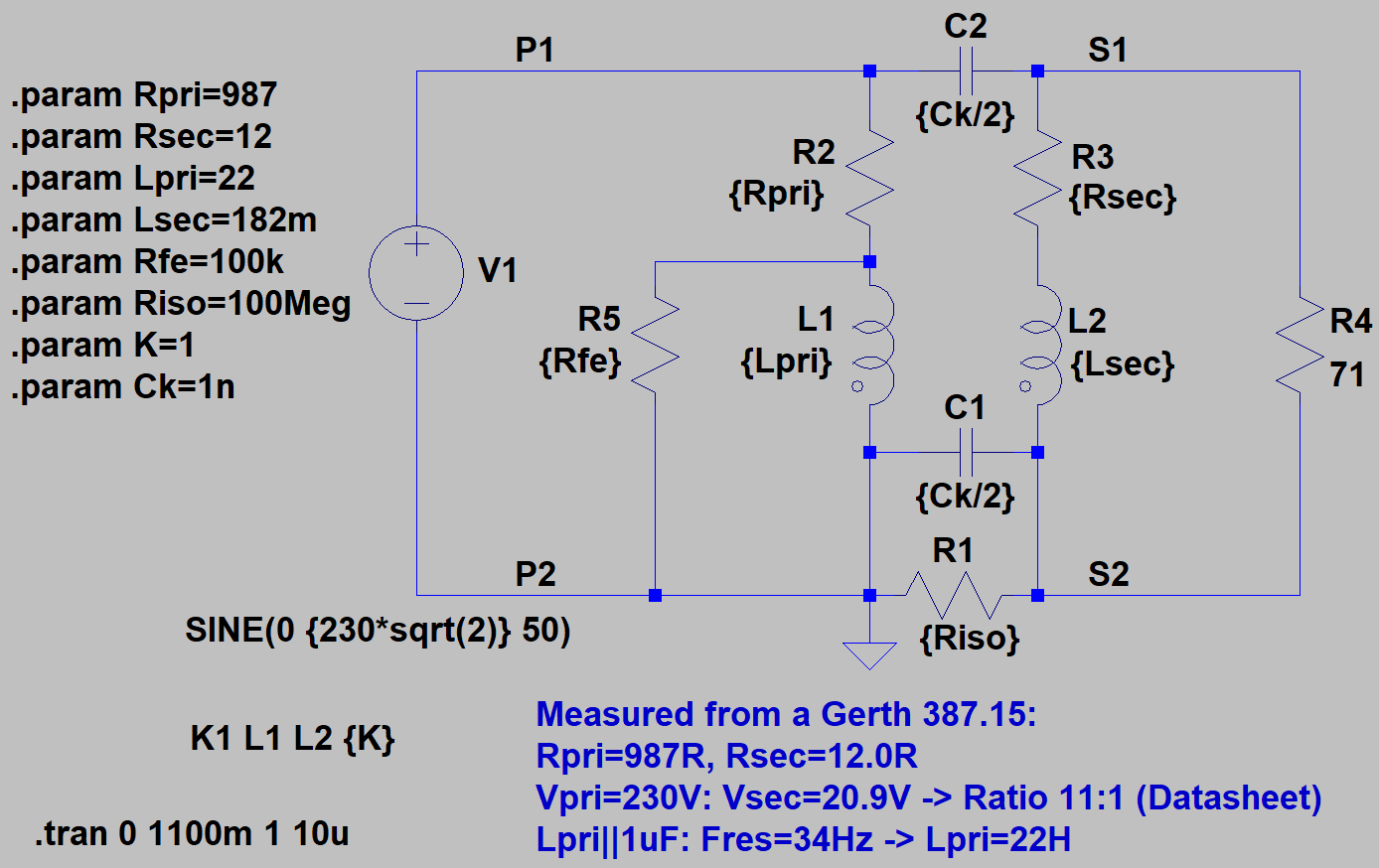 is the simulated transformer circuit. The component values are already defined using parameters, as required for the final model, to allow them to be modified in the top-level schematic.

The 71 Ω resistive load dissipates almost exactly 3.6 W, the transformer's rated power. The effective secondary voltage is 16 V. So, the measured parameters therefore cannot be wildly incorrect...

I must admit, of course, that my method is not ide­al and shouldn't be pushed to the ab­so­lu­te limit. In my defense, this is due in no small part to my inadequate equipment; I have neither a suitable LCR meter nor a wattmeter with sufficient resolution, yet the result aligns quite well with reality and should be good enough for most cases.

I do not wish to repeat myself unnecessarily here. Please consult the section on making own models for details of the procedure.

I saved the model here as a .lib file rather than .sub (the extension makes no functional difference; it is merely a label), because it serves as a prototype for any transformer with a single primary and secondary winding. You can add your own transformers to the same file using the parameters you just measured.

So, here are my symbol and my library (consisting of a single component so far 😆)

Once you have installed the model and symbol in your sub and sym directory, you can try out this test circuit.

You can modify the parameters in your simulations as desired to define your specific transformer, or add it to the xfrm1p1s.lib as I did with the Gerth model, so that you can call it up by name at any time.

I have created this simulation to the best of my knowledge, but I cannot guarantee its ab­so­lu­te accuracy. Use is at your own risk and responsibility.