Monte Carlo Analysis

What you're reading here is actually in the LTSpice help file (just not as nice 😀), but many people are hesitant to try it, probably because of the many parentheses...

I'd like to allay your fears by giving you an example.

As complexity increases, this is often no longer so easy.

A Monte Carlo analysis simulates your circuit many times, each time setting the current values for each individual component to a random value within the specified tolerance. This randomness, like in a roulette game in this famous casino, gave the method its name.

Faites vos jeux!
Les jeux sont faits, rien ne va plus.

So you don't just get one curve for, say, V_out, but a family of curves, and you can see the effects of the tolerances from the extreme values.

Download the circuit and have fun with it!

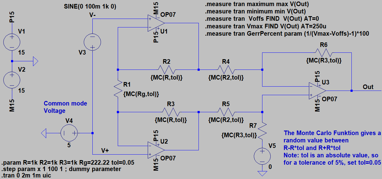
V3 is the input signal. Amplification has been set to 10 by R1. The 100 mV input signal should give 1 V at the output. You may add a common voltage signal with V4. This particularly worsens the offset voltage of the circuit.

Since only resistors determine the behavior in my example, I only have one parameter, tol, which describes the resistance tolerance. In other circuits, you might have an Rtol, a Ctol, and a Ltol, or perhaps even others.

How do you use the Monte Carlo formula?

Normally you would simply specify a value of 10k for a resistor, for example.

If we now want to perform a Monte Carlo analysis, we use the Monte Carlo function instead: {MC(10k,0.05)}. LTSpice then inserts a random value between 10k-(10k*0.05) and 10k+(10k*0.05) for each run of the simulation. The curly brackets tell LTSpice that the expression is not a fixed numerical value, but has to be calculated.

Of course, both value and tolerance can also be a parameter, as we can see in the example, since we have many resistors here that have the same value, and the tolerance can also be adjusted very quickly for all resistors.

To achieve the desired number of iterations, we need a dummy parameter: .step param x 1 100 1. The value x, which here runs from 1 to 100 in steps of one, is not needed anywhere, but the command ensures 100 iterations with newly selected tolerance values each time.

It should be noted that LTSpice works with pseudo-random values here. The 100 values are the same every time the simulation is started. This probably has something to do with reproducibility, but it also means that without this dummy parameter, every simulation produces the same result (and not a new, random one).

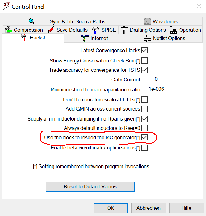
In the settings under Hacks, you can configure the system time to be used to reinitialize the PRNG. This will also give different results for individual simulations.

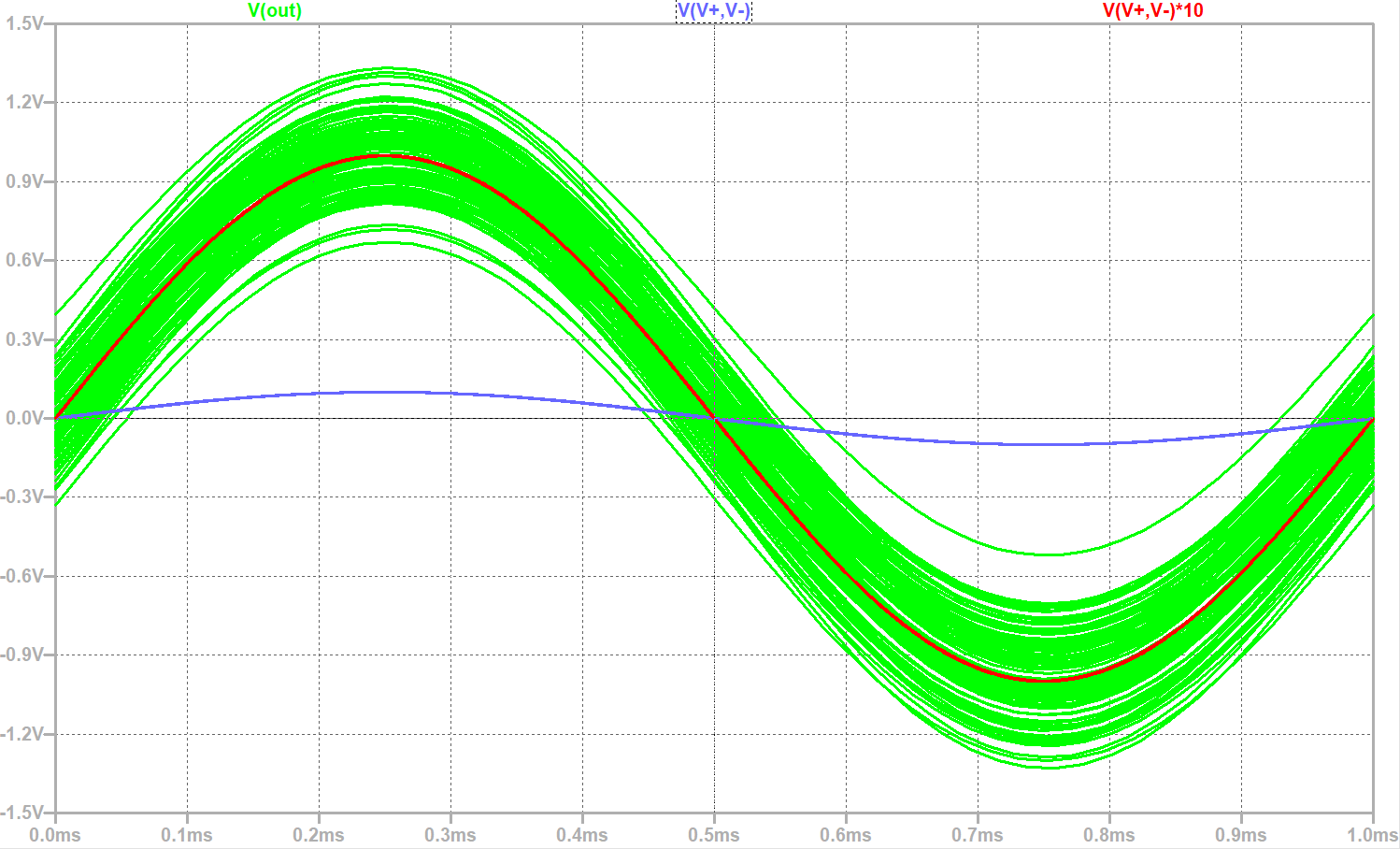Here you can see the result for this deliberately poorly dimensioned circuit with a 5% tolerance, with a common mode voltage (V4) of 5 V and 100 sweeps. While Vout gives an idea of the waveform, the absolute value fluctuates by more than 0.6 V, or almost ±40%! This would be completely useless even for simple measurements.

For illustrative purposes, I have drawn the ideal output signal in red.

Now you also know why you should buy instrumentation amplifiers pre-adjusted and not try to build them yourself. Even with 0.1% resistors, you'd hardly get more than 0.5% accuracy. And that doesn't even take into account the error contributions of the opamps!

And the margins of error?

You have to dig a little deeper for that. At least I haven't found a method to determine them directly.

I've included several .measure statements in this simulation. Of particular interest are the following:
.measure tran Voffs FIND V(Out) AT=0, which calculates the offset error (at t=0, where we would also expect a 0 V output voltage) and:
.measure tran GerrPercent param (1/(Vmax-Voffs)-1)*100, which calculates the gain error in percent.

Both do this for each individual run and I have not been able to directly determine the maximum error from this.

In the Spice Error Log (Ctrl+L or View-Spice_Error_Log) you can see the determined value for each run.

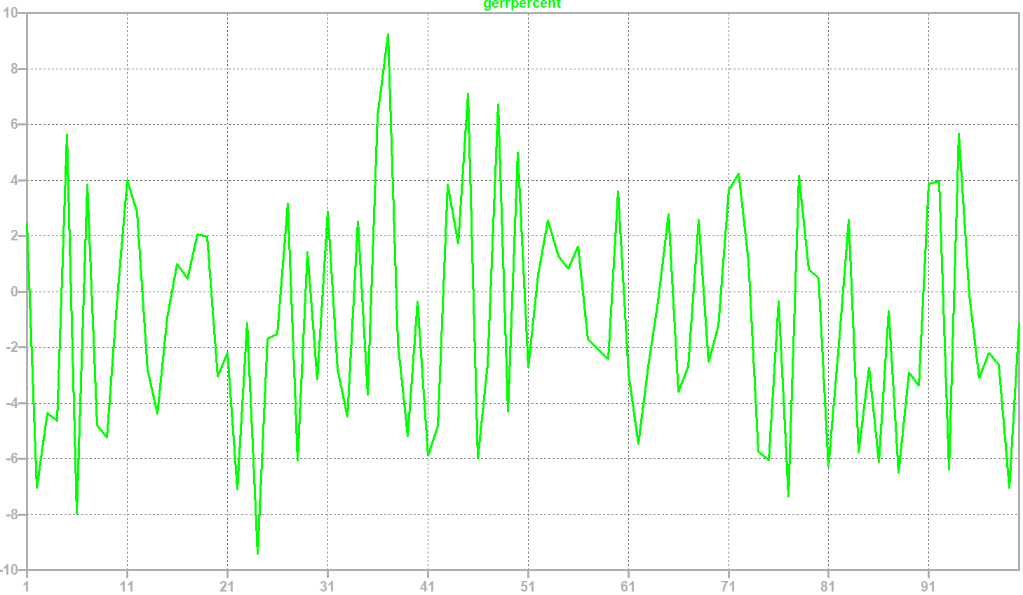
Right-click there and select Plot .step'ed .meas data. A new window will open, and you can right-click again to add the desired curves. The diagram shows an example of the gain error.

You can clearly see here that the maximum error is just under ±10%. The small number of extreme deviations suggests that 100 runs is too small. While it does indicate the direction, if we want to be more precise, we should choose 1000 runs. The simulation times will naturally increase accordingly. 100 runs are certainly sufficient for an initial overview, but if we really want to see the limits, we need to choose significantly more runs—the more, the better. Enough so that at least several extreme values are in a similar range.